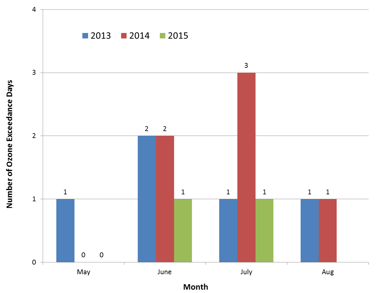
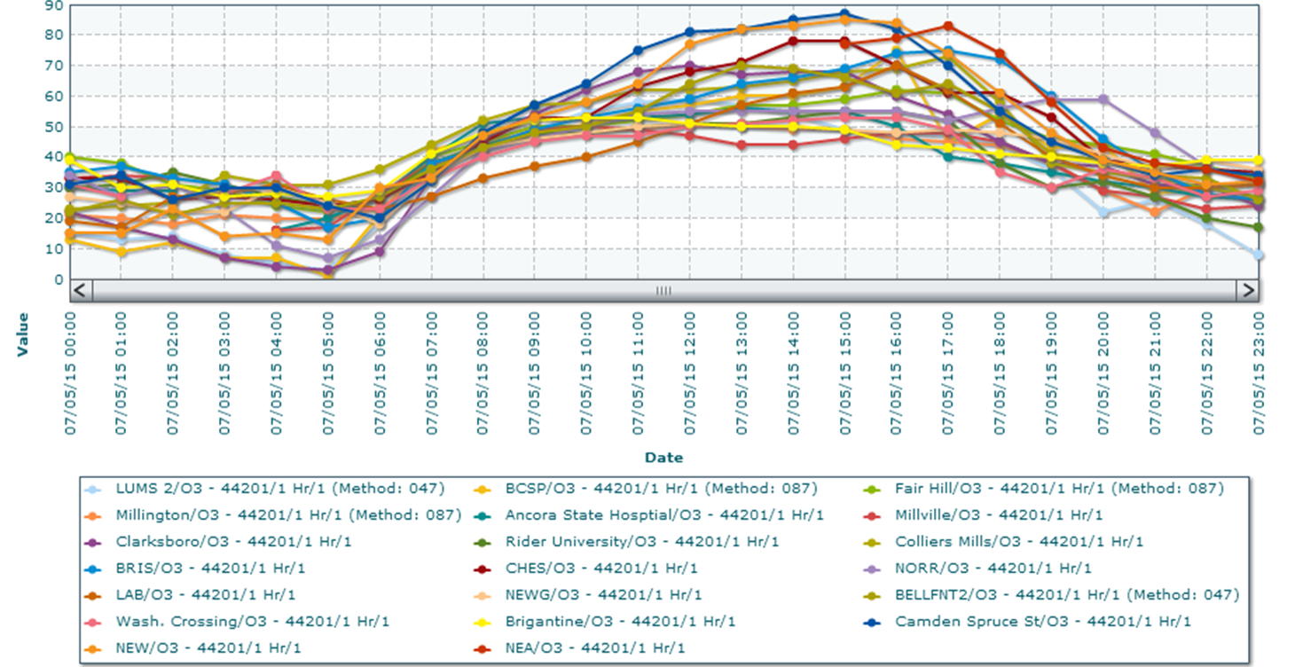
Daily 8-hour average ozone unexpectedly reached the upper Moderate range in northern Delaware on Friday, June 26. The observed maximum 8-hour value was 70 parts per billion (ppb), but we forecasted 50 ppb, for a substantial under-forecast of 20 ppb.  Figure 1 shows ozone beginning to rise around 9 am EDT Friday and continuing to rise throughout the day until 8 pm EDT Saturday. Hourly mixing ratios did not start decreasing significantly until the evening hours.

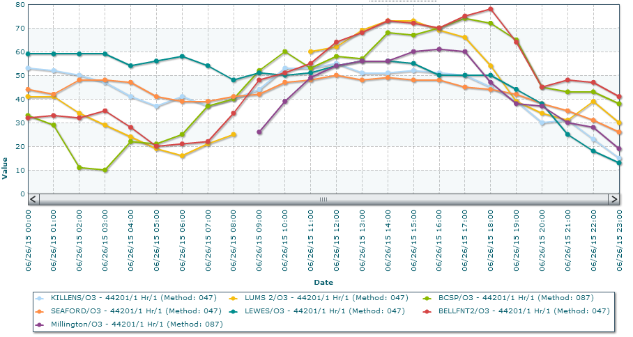
Figure 1. Hourly ozone mixing ratios, in parts per billion (ppb), for Delaware on Friday, June 26, 2015. The red line represents the monitor in Bellefonte, DE, which is the monitor that recorded a daily max 8-hour ozone mixing ratio of 70 ppb. The time along the x-axis is shown in EST, and is offset by two hours. For example, the time stamp of 11:00 represents 1 pm EDT.

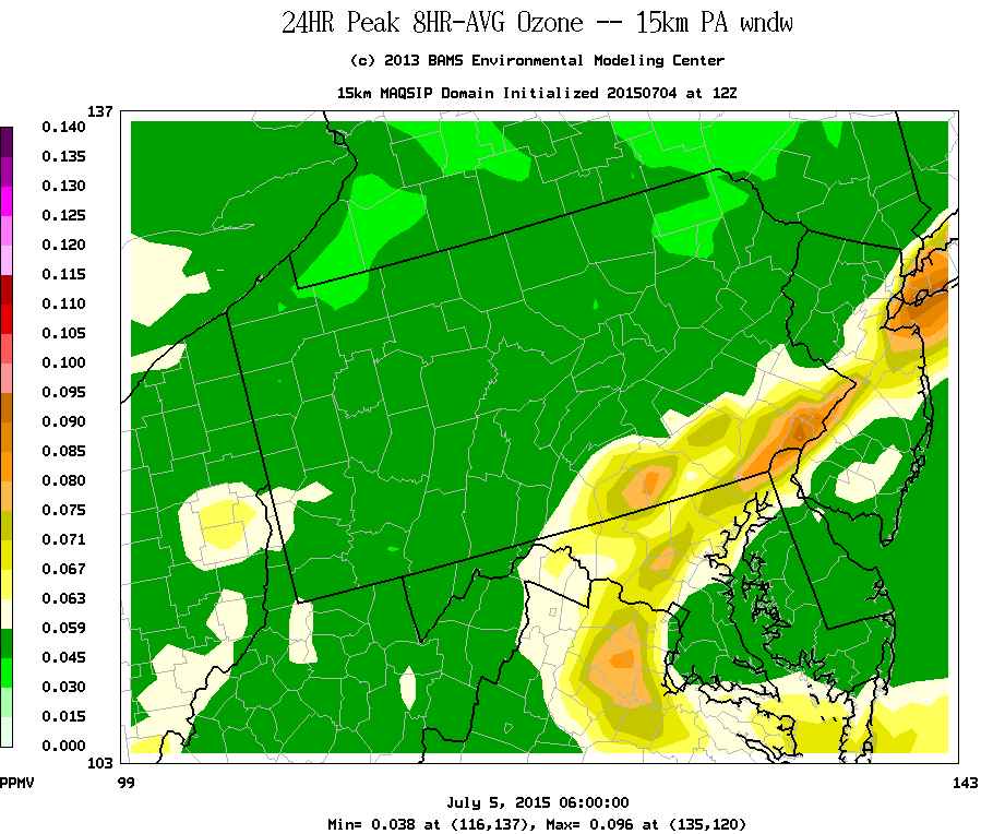
We forecasted Good ozone on Friday in response to widespread clouds and precipitation associated with a stalled frontal boundary in the southern Delmarva and a clean persistence forecast. Most of the air quality model guidance was showing Good ozone throughout Delaware on Friday, with the 12Z NOAA model being the exception. The NOAA model was predicting mid to upper Moderate ozone in northern Delaware, but we deemed its forecast as an outlier (Figure 2). There was high confidence that widespread thunderstorms Thursday evening would clean out the atmosphere of ozone precursors for Friday. Figure 3 shows the heavy precipitation observed on radar Thursday evening. The bulk of the precipitation reached Delaware around 10 pm EDT Thursday as it moved from west to east. The heaviest precipitation was observed in southern Delaware, suggesting that the atmosphere in areas to the north, such as Bellefonte, did not clean out as much as areas to the south. Figure 4 shows the observed precipitation in Dover and Wilmington, respectively. Dover, in central Delaware, observed almost .5 inches more rainfall than Wilmington, in northern Delaware.

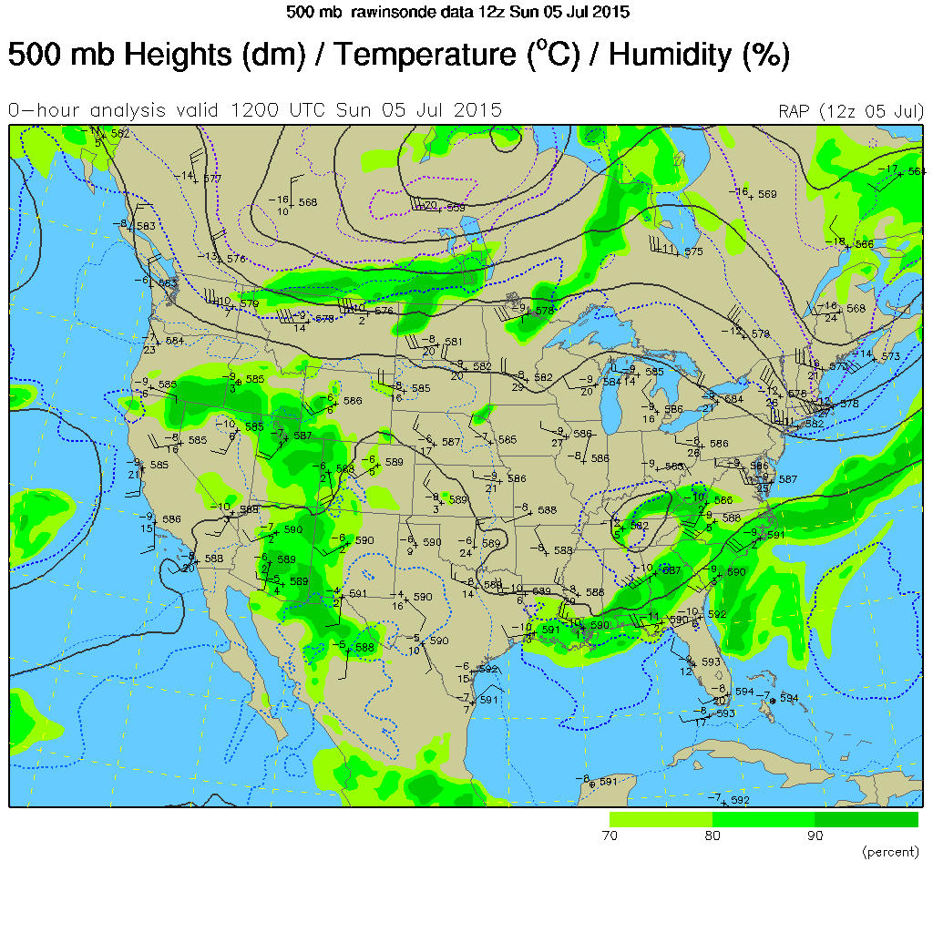
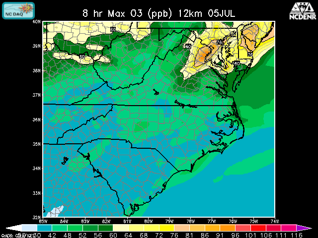
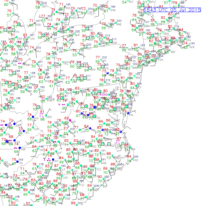
Forecast back trajectories ending at Philadelphia for Friday were showing slight low level onshore transport (Figure 5). Air from offshore locations would have been clean, resulting in a fairly clean residual layer. Our persistence forecast was based on hourly surface observations at 1pm EDT. At this time, many monitors in the area were observing ozone in the upper 40’s to low 50’s ppb, with a few monitors reaching the low 60’s ppb (Figure 6). We put confidence in the persistence forecast, thinking that the transport of the clean air would keep ozone in the Good range in Delaware on Friday. However, our persistence forecast ended up not being very accurate. Hourly surface ozone mixing ratios quickly began to rise after 1 pm EDT, reaching the upper 60’s to low 70’s ppb at 2pm EDT in some locations (Figure 7). Figure 8 shows analyzed back trajectories, ending at Philadelphia at 8 am EDT and 2 pm EDT, respectively. The analyzed back trajectories were different from the forecast trajectories, showing low level transport from the DC Metropolitan area and transport aloft from the Ohio River Valley. These trajectories suggest that there were high concentrations of ozone precursors in the residual layer over Delaware on Friday.

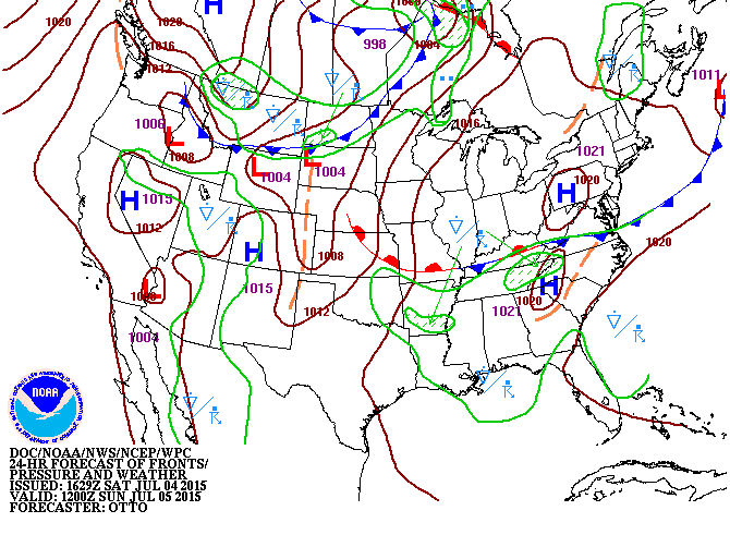
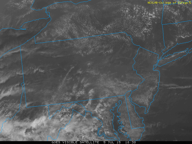
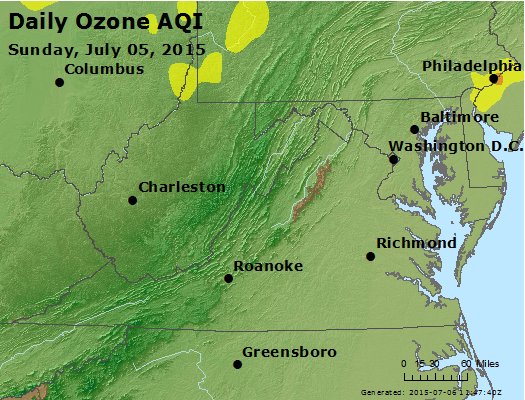
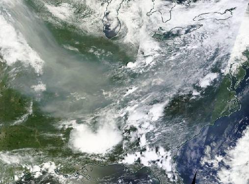
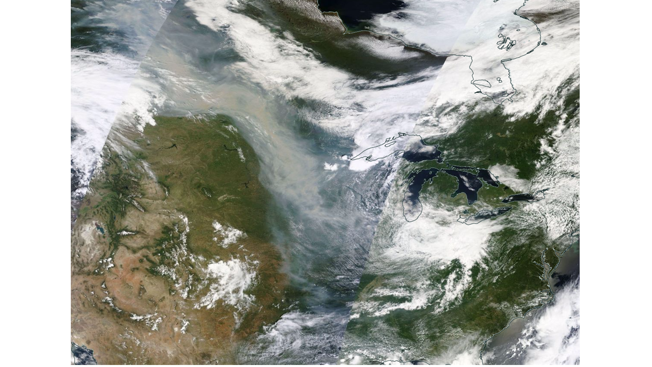
The lack of clearing in northern Delaware and transport of polluted air would not have mattered since overcast skies were expected, effectively shutting down substantial ozone production. Figure 9 shows the widespread cloud cover over the Mid-Atlantic region early Friday afternoon, but there were pockets of clearing over and around northern Delaware. Having just passed the summer solstice, the solar zenith was fairly close to its maximum. This suggests that there was enough sunlight in throughout the day to continue ozone production. If clouds were as thick as they were in Virginia at the time, then ozone production would have likely been limited. In Figure 10, WPC analyzed a center of high pressure over the Chesapeake Bay at 5 pm EDT Friday. The light winds in late afternoon and evening associated with this weak center of high pressure likely contributed to a buildup of ozone in northern Delaware, leading to the small spike in hourly ozone mixing ratios at the Bellefonte monitor in the late afternoon.

Looking back on our forecast, we feel that we put a lot of confidence in the factors limiting ozone production. The forecasted heavy precipitation did not clean out the atmosphere as expected, leading to a more polluted residual layer. Forecast back trajectories were showing clean transport into the region, but we didn’t notice the converging nature of the back trajectories in DC, Dover, and Philadelphia. The late day clearing coupled with long lasting Friday traffic emissions heightened our error even more. We should have been more cautious and banked on the possibility that one, if not all, of these ozone limiting factors would not have verified.

Figure 2. 8-hour average ozone forecast guidance for Friday, June 26 from the 12Z run of the NOAA/EPA model.

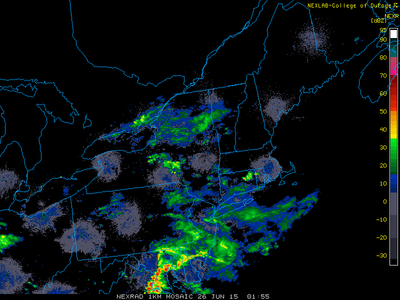
Figure 3. Composite radar reflectivity on the evening of June 25, 2015.

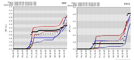
Figure 4. The black dots represent the observed precipitation, in inches, at Dover, DE and Wilmington, DE from Thursday 2 am EDT to Sunday 12 am EDT.

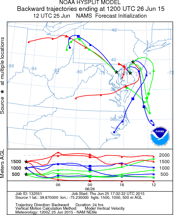
Figure 5. Forecast back trajectories from NOAA’s HYSPLIT Model for Philadelphia, ending at 8 am EDT June 26, 2015.

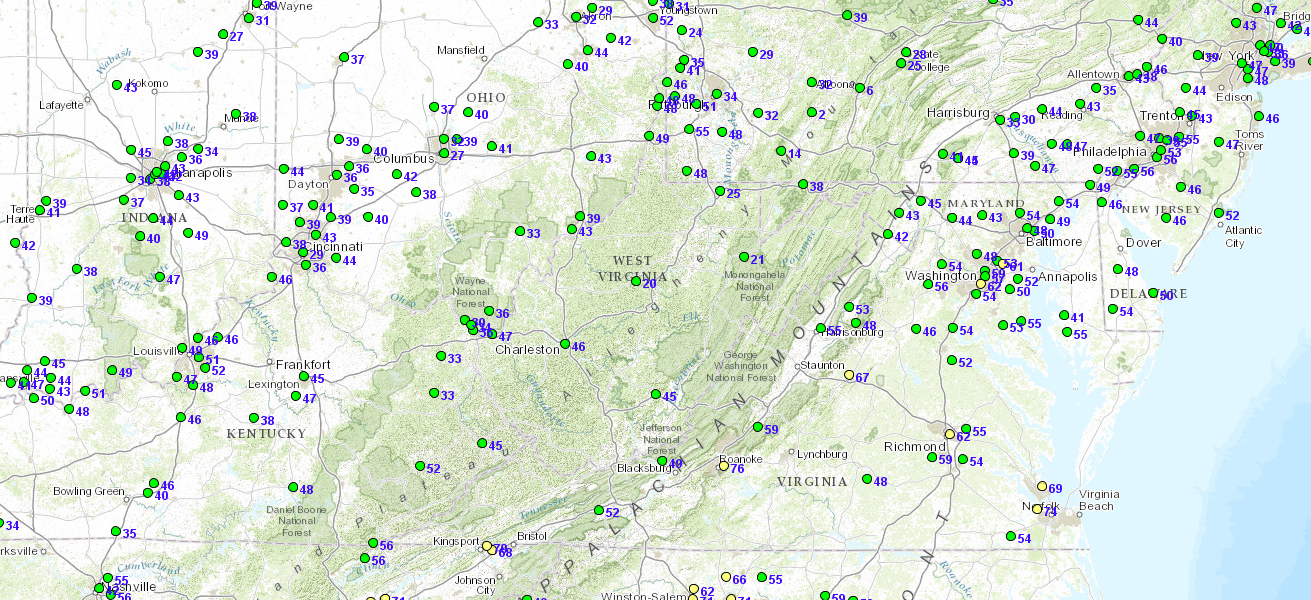
Figure 6. Observed ozone mixing ratios at 1 pm EDT on June 25, 2015 across the Central Mid-Atlantic.

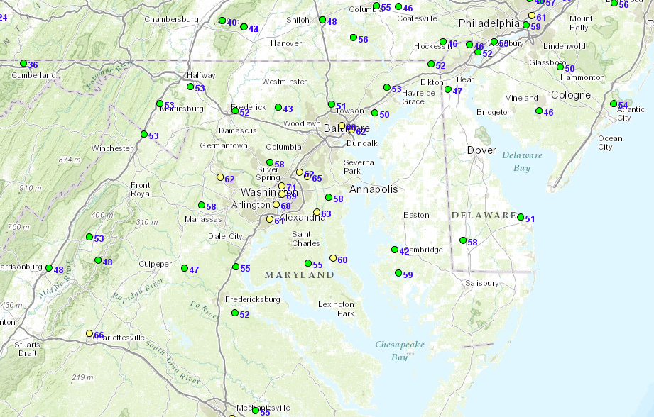
Figure 7. Observed ozone mixing ratios at 2pm EDT on June 25, 2015 in the DC Metro and Baltimore region.

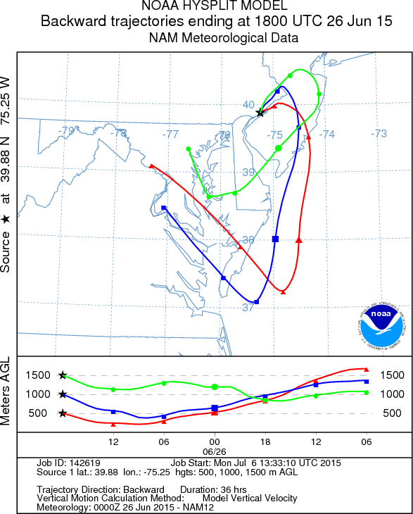
Figure 8. Analyzed back trajectories from NOAA’s HYSPLIT Model for Philadelphia, ending at 2 pm EDT June 26, 2015.

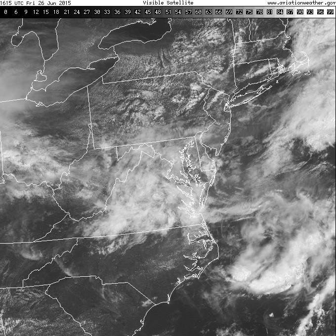
Figure 9. Visible satellite image of the Mid-Atlantic valid at 1215 pm EDT June 26, 2015.

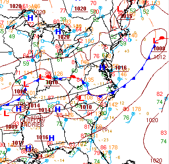
Figure 10. Surface analysis by the WPC at 5 pm EDT with a weak center of high pressure analyzed over the Chesapeake Bay.

By the time we reached the Independence Day holiday weekend, we were overdue for an ozone exceedance day (8-hour average O3 mixing ratio > 75 ppb) in the Philadelphia metropolitan region. This is climatologically the height of the ozone season, when the days are long, the solar zenith angle is short, and daily air temperatures are typically at their peak. Philly has had only one ozone exceedance day so far this summer, however (June 11). This is the farthest we’ve ever gone into the summer without a second exceedance day, even during the recent historically low ozone years of 2013 and 2014. In 2013, we had 1 exceedance day in May and 2 in June, while in 2014, we had no exceedance days in May but 2 in June (Figure 1).

In the week leading up to the Independence Day holiday weekend, the forecasting interns and I had identified Sunday, July 5, as a day of interest for a possible ozone exceedance. The axis of a narrow and fast-moving ridge of high pressure aloft (Figure 2) was forecasted to be just to the west of the Mid-Atlantic, the prime spot for ozone formation. The corresponding center of surface high pressure was forecasted to move across southern PA during the day, promoting sunny skies and calm winds (Figure 3). The main limiting factors were persistence – observed ozone on Saturday was in the Code Green (Good) range across the region – and the fact that it was a Sunday. Historically, lower emissions of ozone precursors on Sundays tend to limit ozone to the upper Moderate range, even when weather conditions are favorable for rising ozone.

All of the air quality models blew up ozone to the Code Orange (USG) range on Sunday (Figure 4). They had excellent consensus with each other and over several consecutive runs (Friday afternoon to Saturday morning). When the air quality models all agree on the location and magnitude of USG ozone, I pay attention. Given the synoptic and mesoscale weather conditions, pockets of USG ozone certainly seemed possible along I-95 from Washington, DC to Trenton, NJ, but I decided that the low regional and upwind ozone on Saturday (low persistence) and the fact that it was a Sunday – even a holiday Sunday – would be enough to limit rising ozone to the upper Moderate range. I thought there was a small chance for isolated USG, but I wasn’t confident enough to issue a USG forecast and call for an Air Quality Alert (AQA). So I forecasted at the top of the Moderate range (74 ppb) for Philadelphia and Baltimore and upper Moderate for DC and Delaware (70 ppb).

It was fascinating to watch the hourly ozone observations come in on Sunday afternoon. Although it was sunny with very light surface winds (Figure 5), 8-hour average ozone stayed in the Good range across Maryland and northern Virginia and barely made it to the Moderate range in northern Delaware (63 ppb). But along a very short section of I-95 in Philadelphia, ozone quickly jumped up at a couple of monitors – Northeast Waste in Philadelphia County and Camden Spruce in Camden County (Figure 6). We ended the day with those two Philly metro area monitors just reaching the USG range for 8-hour average ozone: 76 ppb at Northeast Waste and 78 ppb at Camden Spruce.

This same thing happened last summer – in fact, 3 of the 6 exceedance days in Philadelphia last year occurred under almost exactly the same weather conditions, with Code Green ozone on the previous day, and only 1 monitor reaching USG by 1-2 ppb. So Sunday was not unprecedented, but it was nearly impossible to forecast. I don’t think I could have realistically issued an AQA for the Sunday of Independence Day weekend with the expectation that 1-2 monitors would hit USG by 1-2 ppb. I’m also not sure I could have issued a lower forecast for Maryland… possibly I could have gone lower in the Moderate range, given that it was not forecasted to be as hot, with high temperatures only in the low 80s °F. But I certainly did not expect widespread Code Green ozone (Figure 7)!

Figure 1. Number of observed ozone exceedance days in the Philadelphia metropolitan area by month for 2013-2015.

Figure 2. 500 mb geopotential height analysis at 12Z Sunday, July 5, showing ridge axis to the west of the Mid-Atlantic.

Figure 3. WPC surface analysis forecast for 12Z Sunday, July 5, showing the center of surface high pressure over western PA.

Figure 4. 8-hour average ozone forecast guidance for Sunday, July 5 from the 12Z runs of the NOAA/EPA model (top), BAMS-MAQSIP model (middle), and NCDENR model (bottom).

Figure 5. METARS surface observations at 18:45 UTC (top) and GOES visible satellite image at 18:30 UTC (bottom).

Figure 6. Time series of hourly ozone observations for the Philadelphia/Trenton/Wilmington metropolitan region for Sunday, July 5.  Note the topmost lines for Camden Spruce (dark blue) and Northeast Waste (NEW; orange).

Figure 7. Observed ozone AQI color codes for the Mid-Atlantic region for Sunday, July 5.

Updating yesterday’s post, it appears that the fire smoke from the large group of fires in western and central Canada is continuing to work its way into the eastern US and will impact the mid-Atlantic region in the next few days.

Yesterday’s polar orbiter images via MODIS shows the extent of the smoke:

This morning’s PM2.5 surface observation show high concentration in KY and beginning to increase at the high elevation monitor at Big Meadows, VA in Shenadoah NP.

Figure 1.  PM2.5 hourly concentrations at Big Meadows, and two monitors in KY, July 1.  Data courtesy of EPA AirNow.

The long Western drought and the recent extremely hot and dry weather have resulted in widespread wildfires from Alaska, through the Pacific Northwest, and into Canada.  At this time, smoke from a group of wildfires centered in northern Alberta have begun to push southward into the United States.

  Figure 1.  Map of wildfire locations in Canada, courtesy of the Active Fire Mapping Program, http://activefiremaps.fs.fed.us/ (upper left). Visible image of northern Alberta from MODIS aboard Aqua, June 28, 2015 (lower right).

By yesterday, Monday, June 29, the smoke plume can be clearly seen across the upper Midwest (Figure 2). The questions of most interest are the future direction of the smoke and whether it will mix downward to the surface.  Smoke plumes from strong wildfires are typically lofted upward near their source and may remain well aloft, not interacting with the surface, for long periods.  As of this morning, surface PM2.5 observations show that some of the smoke has impacted ground level observations sites (Figures 3 and 5).  The future path of the smoke is related to the large scale weather pattern which features a trough of low pressure over the eastern US (Figure 4).  This means that the smoke in the upper Midwest will move in a counter-clockwise arc towards the east.  Upward motion over the Ohio River Valley and northward should keep the smoke well above the surface, but this cannot be said for areas of smoke that drift further south.  This analysis suggests that smoke will impact the southeastern  US on Wednesday and perhaps the mid-Atlantic on Thursday.

Figure 2.  Visible satellite image from June 29, 2015.

Figure 3.   AirNow Navigator PM2.5 observations, June 30.  Blue shaded area is the area of fire smoke currently observed by surface-based PM2.5 monitors.  The arrows are rough estimates of the expected track of the smoke plumes.  The dashed line tracks the northern path where upward motion is expected.  The red line tracks the southern path characterized by less upward motion and more likely surface impacts.

Figure 4.  500 mb geopotential heights, winds and humidity, June 30, 2015.  Winds are roughly parallel to the isoheight lines.

Figure 5.  Satellite estimated PM2.5 concentrations, June 29, 2015. http://www.star.nesdis.noaa.gov/smcd/spb/aq/index.php?product_id=2

US EPA recently launched a new air quality outreach project called Village Green. The project involves placing air quality monitoring stations in local communities across the country. The monitoring system is built into a park bench and includes measurements of basic meteorological conditions (e.g., air temperature, relative humidity, wind speed/direction) as well as O3 and PM2.5 concentrations. The pilot Village Green station is located outside of the South Regional Library in Durham, NC. One of my friends lives in Durham and sent me a photo of the station (below). These stations are designed for education and outreach, so they are not used for regulatory purposes. One of the most recent stations to join the project is located in downtown Philadelphia, in Independence National Park near the National Constitution Center. This station is being administered by the Air Management Services (AMS) division of the Department of Public Health of the City of Philadelphia in partnership with US EPA. There was a ribbon cutting ceremony for the station on May 1, to coincide with Air Quality Awareness week. You can find the current weather and air quality observations from the Philadelphia Village Green station here. Congratulations to AMS and US EPA for bringing this exciting new outreach project to Philadelphia! Anything we can do to raise awareness of air quality is a great thing.

Thanks to Kerrie Schmehl for the photo of the Durham Village Green Station.