Category Archives: Blog Posts

PSAQFO Student Meteorologist Matt Brown Featured in Penn State News Story

Matt Brown, recent PSU Meteorology graduate and summer forecasting intern with the PSAQFO, was featured in an October Penn State News story. Matt (below) worked with Dr. Amy Huff and Bill Ryan during summer 2016, forecasting daily ozone and PM2.5 air quality for Philadelphia and the State of Delaware. Matt is currently in his first year of a MS program at Texas A&M University.

matt_photo

August 2016 Warmest on Record for Philadelphia but Only One Ozone Exceedance Day Observed – August 31

According to the Mt Holly National Weather Service (NWS) Office, August 2016 was the warmest August in Philadelphia, based on records dating back to 1874, with an average high temperature of 81.1 °F, which is almost 4 °F higher than the 30-year normal of 76.6 °F. In August, KPHL had 17 90 °F days, compared to a mean of 5 days, while KILG had 15 90 °F days, also relative to a mean of 5 days. Despite this record warmth, and plenty of sunshine, there was only one ozone exceedance day this month in Delaware (August 27 – see my previous post) and only one in Philadelphia – yesterday, August 31. This underscores the breakdown in the relationship between hot weather (90 °F days) and high ozone in the past ~4 years: we still need very warm to hot weather (Tmax ≥ 85 °F) for high ozone, but only a small fraction of all hot days are exceedance days. The hard part is determining which of the many hot and sunny days will be conducive for high ozone.

After getting a rough start forecasting the 2016 ozone season, we acclimated in August, with no false alarms or missed forecasts, and a forecast hit for the 31st. I had lower than normal confidence in the forecast for the 31st, but a variety of ozone-conducive factors were in place. The region was pre-frontal, with a strong cold front approaching from the northwest. Clouds and thunderstorms associated with the advancing front were expected to hold off through the late afternoon, keeping Philadelphia under full sun, which verified (Figure 1; click on figures to enlarge). At the same time, Tropical Depression Nine was lurking off of the coast, southeast of the Delmarva. The National Hurricane Center had expected to TD9 to strengthen into Tropical Storm Hermine, but it did not. A nearby tropical cyclone can be tricky for air quality forecasts because strong subsidence ahead of the storm can enhance ozone formation, as long as the cyclone is not so close that its clouds or tropical air impact the forecast area. I had been concerned that a possible TS Hermine might provide a boost of subsidence for locations along the I-95 Corridor, but the weaker TD9’s subsidence ended up being concentrated offshore (Figure 1).

It turned out that there was enough afternoon sun and surface convergence from weak southwesterly winds along I-95 (Figure 2) for the four most northwesterly monitors in the Philadelphia forecast area to exceed, with a maximum observed 8-hour average of 80 ppbv at the Bristol and Northeast Airport monitors. Two monitors in the Baltimore metro area also exceeded, as well as several in southwestern CT. There was enough onshore flow to keep the northern Delaware monitors in the upper Moderate range, as forecasted, as well as most of NJ, with only the Camden monitor, located just across the river from Philadelphia, recording an exceedance. So most of the forecasts for the day verified (Figure 3), which was a great way to close out the month.

add_BWI_vis
Figure 1.  GOES visible satellite imagery for the Mid-Atlantic at 1607UTC on August 31, 2016

sfc_bwi_16UTC sfc_bwi
Figure 2.  METARS surface analysis for the Mid-Atlantic for 1628 UTC (left) and 2225 UTC (right).

NWS_Watches-Warnings_20160831 peak_o3_ny_pa_nj_20160831
F
igure 3. Forecasted ozone exceedance regions (left) and observed exceedances (right) for August 31, 2016.


Surprise Ozone Exceedances in Wilmington on August 27

Ozone unexpectedly exceeded the daily NAAQS of 70 ppbv on Saturday at two monitors in Wilmington, DE: MLK (73 ppbv) and Bellefonte (71 ppbv). The only other monitor along the I-95 Corridor that exceeded was the nearby Fair Hill, MD monitor (75 ppbv). Figure 1 shows the daily ozone AQIs for the region (click on individual figures to enlarge).

The exceedances were a surprise because the region was post-frontal (Figure 2), with what had seemed on Friday to be a relatively clean air mass in place. I think that was true, given the essentially isolated nature of the exceedances. The NOAA model guidance for Saturday (Figure 3) had indicated the possibility for ozone exceedances along the Fair Hill-Wilmington-Chester stretch of I-95, but the NOAA model had been over-forecasting consistently for the past three weeks, and the other air quality models predicted Moderate ozone, so I undercut the guidance. That was the right call for Chester, where daily ozone only reached 66 ppbv (right in line with my forecast of 65 ppbv), but not in Wilmington.

So what went wrong? There was a strong ridge in place (Figure 4), with the center directly overhead, which promoted stagnation. It was sunny all day (Figure 5), with temperatures reaching 91 °F at KILG, and slightly lower humidity than in recent days (dew points were hovering around 60 °F at KILG). Surface winds were light all day and recirculated from the north in the morning (Figure 6a) to the east/southeast (Figure 6b) in the afternoon. I think the two Wilmington monitors (and the Fair Hill monitor) were in a “sweet spot” of surface convergence that kept I-95 highway emissions localized enough to promote abundant sustained afternoon ozone production. The exceeding monitors had fairly steady high hourly ozone from 2 PM all the way through 7 PM, whereas hourly ozone values at neighboring monitors were either slower to rise or quicker to drop off.

I’m not sure what I could have realistically done differently with the forecast. In my many years of forecasting for the Mid-Atlantic, I can’t recall ever seeing a situation like we had on Saturday – in which two Wilmington monitors exceeded but not any in Philadelphia, under afternoon onshore flow (albeit light) and absent any strong mesoscale convergence feature like a weak frontal boundary or sea breeze. Part of it is inexperience with the new ozone standard – Saturday would not have been an exceedance day under the previous daily NAAQS of 75 ppbv. I will also have to remember that light northerly flow aloft with recirculating surface winds, like we had on Saturday, can be an issue for northern Delaware, particularly with a mid- or upper-level ridge overhead.

peak_o3_ny_pa_nj_20160827
Figure 1.  Daily peak ozone AQI values for Saturday, August 27.

WPC_18Z_20160827
F
igure 2.  WPC surface analysis for 18 UTC on August 27, showing a stalling cold front well south of the Delaware forecast region.

12Z_NOAA_O3_20160827
Figure 3.  NOAA-EPA model guidance for August 27.

12Z_eta500_vrt_20160827
Figure 4.  500 mb analysis for 12 UTC on August 27.

add_BWI_vis
Figure 5.  GOES visible satellite imagery for the Mid-Atlantic at 16UTC on August 27.

sfc_bwi_amsfc_bwi_mid
Figure 6.  METARS surface analysis for the Mid-Atlantic for 1255 UTC (a) and 1625 UTC (b)


Checking in on the 2016 Ozone Season: the Recent Downward Trend in Observed Ozone Continues

Now that we are almost 80% of the way through the 2016 ozone season, it seems like a good time to check in and see how things are progressing. Back on May 20, I wrote a post on the outlook for the 2016 season. We were very interested to see how this year’s ozone season would stack up to the previous three seasons, during which we saw a sudden and very dramatic decrease in observed ozone levels compared to the period 2003-2012. Based on this recent downward trend, and taking the new ozone NAAQS into account, we predicted about 18-22 exceedance days in Philadelphia and 6-8 days in Delaware for the 2016 ozone season. Exceedance days occur when observed 8-hour average ozone is ≥ 71 ppbv.

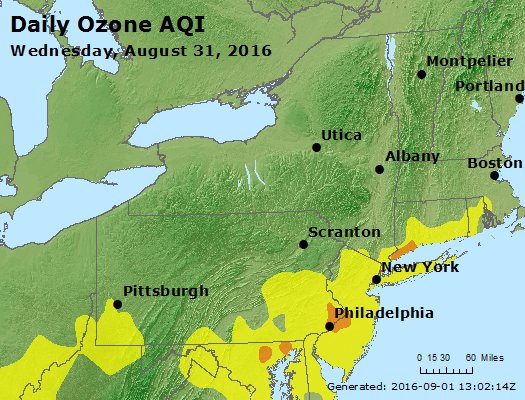
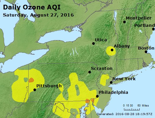
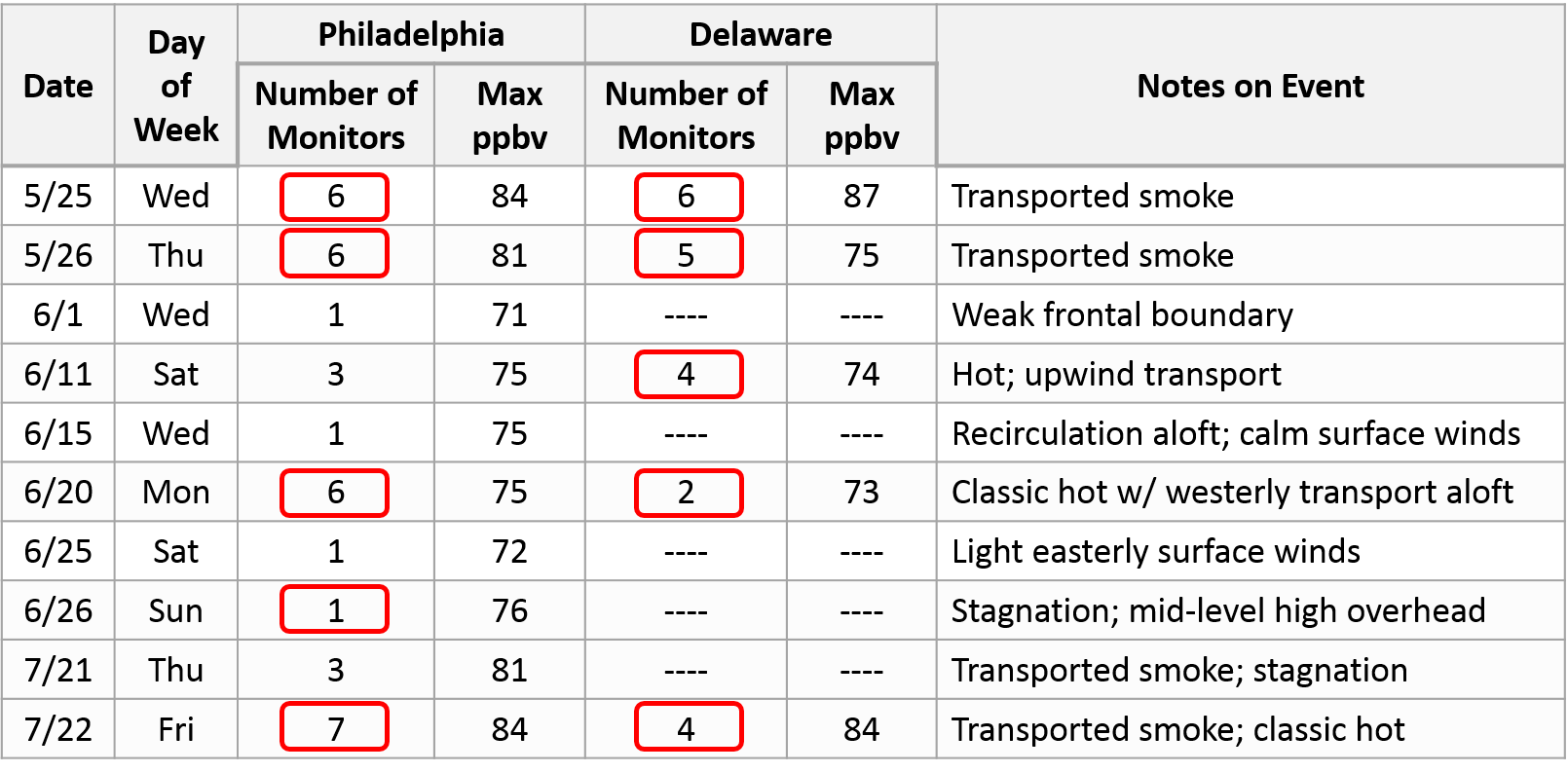
Table 1 (click on table to enlarge) shows that we are well behind our predicted average for 2016 in Philadelphia (10 exceedance days so far) but just about on pace in Delaware (5 days so far). The red rectangles in Figure 1 indicate the days for which we correctly forecasted the ozone exceedances. We are doing really well in Delaware, having correctly identified all of the exceedance days so far this season and issuing only three false alarms. (To be fair, I should acknowledge that officially, there have been two additional exceedance days in Delaware, but they were what Bill and I consider technicalities, in the sense that they were validated at one monitor with only 6 continuous hours of data. While these two days technically count as exceedances from a regulatory standpoint, I contend that they don’t count from a health/forecasting perspective.)

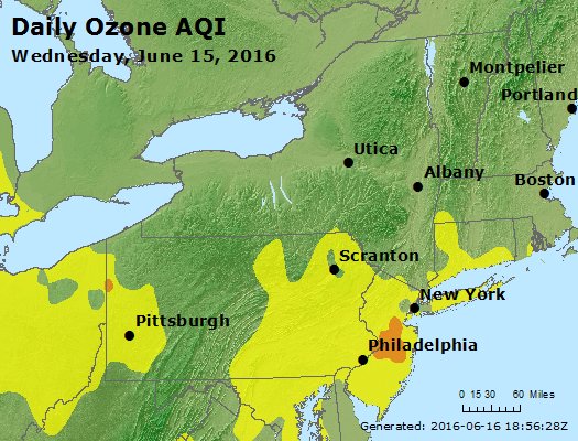
In Philadelphia, however, we are not doing so well; we have only identified half of the exceedance days. Note that three of the days we missed were localized events (June 1, 15, and 25), with only one monitor exceeding by a few ppbv, driven by mesoscale weather conditions that are inherently difficult to predict. The exceptions are June 11, when we had high ozone transported from upwind on the first 90 °F plus day of the summer (see my previous post), and July 21, when transported smoke and local stagnation combined to push observed 8-hour ozone up to 81 ppbv, with exceedances at three monitors. The other main problem in Philadelphia is that we’ve issued a whopping seven false alarms, most of which have been epic fails (7-11 ppbv too high).

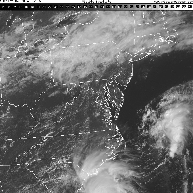
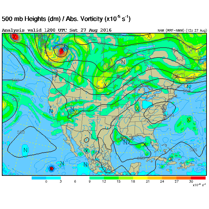
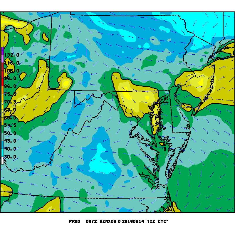
The five missed exceedance days and preponderance of false alarms in Philadelphia underscore the challenges of identifying which days will be high ozone days. Concurrent with the recent drop in observed ozone beginning in 2013, we’ve seen a shift in the main meteorological factors that lead to high ozone. Historically, high ozone days in the Mid-Atlantic were characterized by synoptic conditions including hot weather (Tmax ≥ 90 °F), westerly transport aloft from the Ohio River Valley, a strong ridge of high pressure aloft, and slowly migrating high pressure at the surface. These conditions led to more widespread, multi-day high ozone events. So even if we missed the onset day, we could reasonably forecast the remaining days in an event. Now, high ozone days are driven primarily by mesoscale features, such as weak frontal boundaries, stagnation, and bay/sea breezes. We still seem to have a few days that fit the more “classic” mold, such as June 20 and July 22, but they tend to be single day events. And by no means is hot weather a guarantee of high ozone anymore… for example, we had an extremely hot July, but only two exceedance days in Philadelphia and one in Delaware. We haven’t had an exceedance day in either forecast area in the past month, despite persistent above average temperatures during most of that period. And both of the exceedance days in July were influenced by transported wildfire smoke, which seems to be the real wild card in recent years. At least for Philadelphia and Delaware, the highest ozone we see now is associated with transported smoke, such as on May 25-26 and July 21-22. Yes, July 22 was influenced by “classic” hot conditions, but ozone reached up into the low 80s ppbv (instead of peaking in the 70s ppbv) due to the presence of smoke.

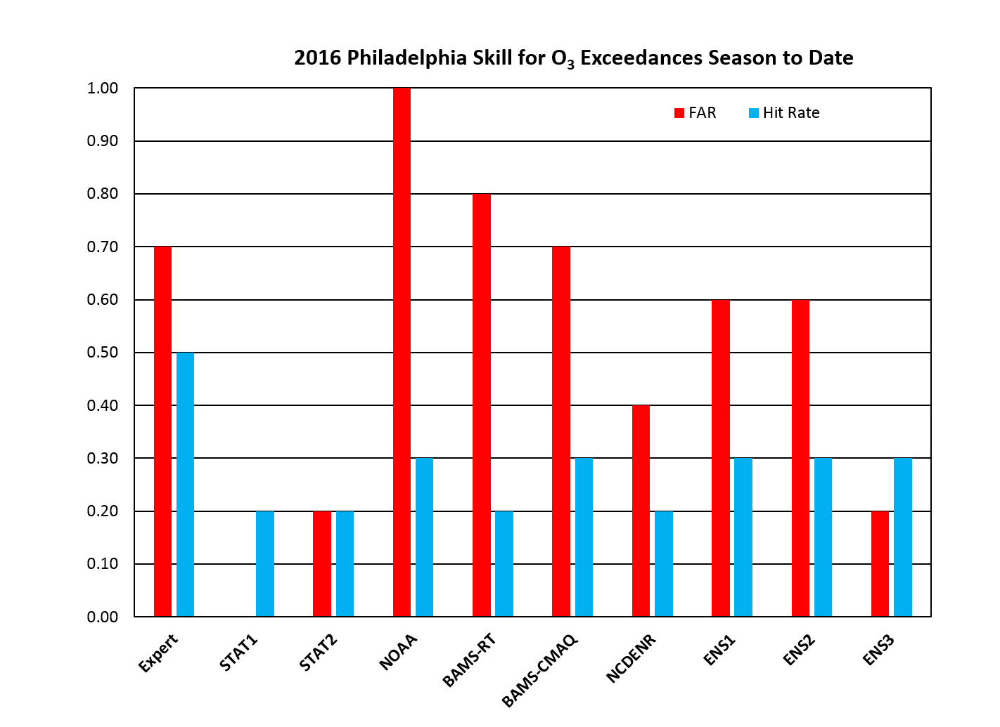
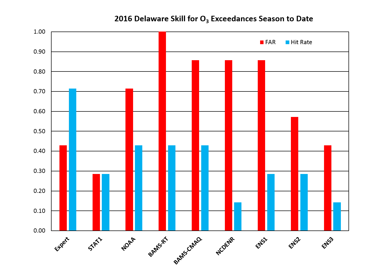
And we can’t rely on the air quality models to help us identify the exceedance days. Figures 1 and 2 (click on figures to enlarge) show the skill scores (hit rate and false alarm rate) for ozone exceedance days in 2016 for Philadelphia and Delaware, respectively. You’ll notice that across the board, the false alarm rate is higher than the hit rate for all of the numerical model guidance, and the “expert” forecasts have higher skill than any of the model guidance. Also included in Figures 1 and 2 are the skill scores for our updated statistical models, which include variables such as maximum temperature, surface wind speed in the morning, and relative humidity in the afternoon. Due to the lessening influence of synoptic weather conditions, the updated statistical models are not really helping us much this year, either, although they have some promise for helping to avoid false alarms.

The take home message is that the recent “step-down” in observed ozone seems to be here to stay, and it is not an anomaly due to fluctuating meteorological conditions over the past three summers. We can presumably look forward to a continuation of fewer ozone exceedance days in the next few years, relative to the 2003-2012 average. At the same time, correctly forecasting these days remains more of a challenge than ever, due to the weakened correlation between hot weather and high ozone, as well as the shift to predominantly mesoscale-driven ozone conducive conditions.

Ex_Table_20160826
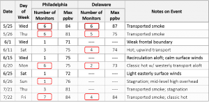
Table 1.  Observed ozone exceedance days for the 2016 season to date in the Philadelphia and Delaware forecast areas.  The red rectangles indicate days when the exceedance was correctly forecasted.

PHL_SS_20160826
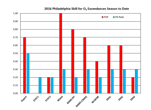
Figure 1.  Skill scores for ozone exceedances for the Philadelphia forecast area.  The best hit rate is 1.0 and the best false alarm rate is 0.0.  The numerical ozone models include “NOAA” (NOAA-EPA model), “BAMS” (Barons Meteorological models), and “NCDENR” (North Carolina model).  “STAT” refers to statistical models, and “ENS” indicates various “ensemble” averages of different combinations of the numerical and statistical guidance.

DE_SS_20160826
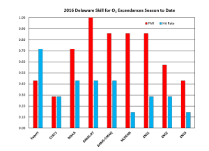
Figure 2.  As in Figure 1, but for the Delaware forecast area.


Isolated Ozone Exceedance in Philadelphia Metro Area on June 15: Is It Time to Seriously Consider Morning Forecast Updates?

Ozone exceeded the 70 ppbv NAAQS in an isolated area of northeastern PA (one monitor) and central NJ (2 monitors) on Wednesday, June 15 (Figure 1). The exceeding Philadelphia forecast region monitor was Bristol, at 75 ppbv for the 8-hr average; in NJ, the Rider University and Colliers Mills monitors both just exceeded at 71 ppbv for the 8-hr average. This isolated area of USG ozone was courtesy of localized and recirculating back trajectories (Figure 2), calm surface winds, and essentially full afternoon sunshine (Figure 3). This combination was sufficient, in conjunction with Philadelphia metro area emissions, to push ozone into the USG range.

What is interesting (and troubling) about this event is that it wasn’t what we consider “hot enough” for USG ozone – high temperatures only reached 83 °F at KPNE, the closest ASOS station to Bristol, while maximum temperature was 79 °F at KPHL (Figure 4). Historically, we don’t see USG ozone along the I-95 Corridor until temperatures reach a minimum of 85 °F on the urban scale. The temperature gradient between KPNE and KPHL was due to a line of clouds that covered Delaware and the southern and western portions of the Philly metro area (Figure 3), but didn’t extend far enough to the north to cover the Bristol monitor. We expected these clouds, but we thought they would cover the entire Philly forecast area (Figure 5) and keep ozone in the upper Moderate range. The other interesting (and troubling) aspect of this exceedance was that, for the second time this season, ozone went from Good to USG the next day. The observed 8-hr ozone maximum in Philadelphia on June 14 was 54 ppbv. It used to be extremely rare to go from Good to USG ozone in 24-hours, but it’s become increasingly common in Philadelphia in the past couple of years. So once again, we can’t rely on persistence as a forecast tool. We knew the air mass was going to be somewhat stagnant, but it was relatively clean on June 14, with estimated upwind persistence in the mid-50s ppbv for the 8-hr average. Typically, we look for upwind persistence in the mid-60s to 70s ppb for the 8-hr average at a minimum to get us to USG in Philly, in conjunction with local ozone production.

Once again, the air quality models did not pick up on this event. The NOAA model guidance (Figure 6), as a representative example, sort of had a bulls-eye of Moderate ozone in the correct place in central NJ, but the magnitude was low, and the other bulls-eye in the DC/BAL area was much too high and didn’t verify.

So far this season, we haven’t been able to rely on any of our usual forecasting “tools” to predict USG ozone. This event demonstrates that temperature isn’t very reliable anymore, and persistence has been a weak forecast variable all season (and last season too). The air quality models aren’t even helping us. So where do we go from here? In retrospect, given the information I had on Tuesday afternoon, I would not have been justified in issuing a USG forecast for Philadelphia for Wednesday. However, on Wednesday morning, it was obvious that the air mass was modified, with a lot of NOx titration, and I could see the line of clouds was not reaching over the northern suburbs, as expected. At that point, I could have updated the forecast to USG, but we don’t have a mechanism in place in PA to do so. I think it’s time for us as a community of Mid-Atlantic forecasters to consider being able to issue morning updates to our forecasts. I brought this idea up with some colleagues last year, and it’s fraught with complications, especially in the Washington, DC metro region, since AQA alerts trigger actions related to transportation and health across multiple state and local jurisdictions. As a result, enacting or cancelling an AQA “the day of” (instead of the day before) does not provide enough lead time for transportation/health actions and warnings/messaging (like on highway signs). But given the increasingly localized nature of emissions across the region, and the growing importance of mesoscale weather features, not synoptic, for air quality conditions, it’s becoming clear that we often can’t accurately predict ozone levels the day before.

peak_o3_ny_pa_nj_20160615
Figure 1.  Observed ozone AQI values for Wednesday, June 15.

12Z_NAM_PHL_24hr_12Z_20160615
Figure 2.  24-hour back trajectories ending at KPHL on June 15 at 12 UTC.

CODNEXLAB-1km-NJ_Penn_vis_20160615_1900-100-100-raw
Figure 3.  GOES visible satellite image for June 15 at 19 UTC.

WPC_SfcAnalysis_crop_18UTC_20160615
Figure 4.  WPC surface analysis with station data for June 15 at 18 UTC.

12Z_NAM_4km_clouds_23Z_20160615
Figure 5.  Clouds and precipitation guidance from the 12 UTC run of the 4 km NAM for June 15 at 23 UTC.

12Z_NOAA_O3_20160615
Figure 6.  8-hr average maximum ozone guidance for June 15 from the 12 UTC run of the NOAA model on June 14.